6. Basics of Optimization #
Paolo Bonfini, 2025. All rights reserved.
This work is the intellectual property of Paolo Bonfini. All content produced in this notebook is original creation of the author unless specified otherwise. Unauthorized use, reproduction, or distribution of this material, in whole or in part, without explicit permission from the author, is strictly prohibited.
This notebook introduces to the concept of “optimization”, in the sense of finding the best parameters of a function.
Notice that “optimization” is an umbrella term, which, depending on the specific context, can manifest as:
minimization
maximization
fitting
In this notebook, we will focus on function fitting, but the concepts outlined here are valid for optimization in general.
For the sake of this course, we can use the terms “fit” and “optimize” interchangeably
7. What is [parametric] fitting#
Easiest to start with a linear example.
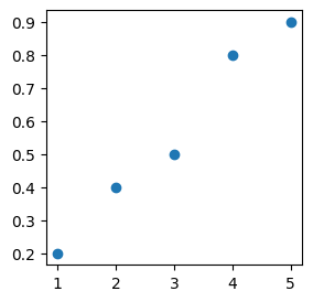
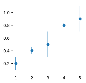
Say we have some observed data:
X = [1, 2, 3, 4, 5]
y = [0.2, 0.4, 0.5, 0.8, 0.9]

from matplotlib import pyplot as plt
plt.figure(figsize=(3,3))
plt.scatter(X, y)
plt.show()
… and we want a model that represents the true beahvior of the data.
We may want to use it for:
predicting new data
explain the phenomenon that causes our observations
Let’s assume a one-dimensional linear model, that is, a model of the type:
where we call \(\alpha\) and \(\beta\) the model parameters.
By changing the parameters we obtain different models, e.g.:
import numpy as np

def funct(xx, alpha, beta):
    return alpha*xx + beta

xx = np.linspace(0 ,5, 100)
'''Notice that `xx` is not the same as `X` (the data), but just
an array of equally spaced values that we use for plotting purposes.'''

alphas = [0.1, 0.27, 0.05]
betas  = [0.2, -0.2, 0.3]

plt.figure(figsize=(3,3))

for i, (alpha, beta) in enumerate(zip(alphas, betas)):

    y_model_i = funct(xx, alpha, beta)
    plt.plot(xx, y_model_i, label='model %s' % i, c=str('C%s' % (i+1)))

plt.scatter(X, y)
plt.legend()
plt.show()
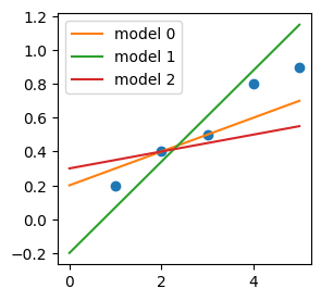
It is convenient to think that each parameter set gives rise to a different model
(\(\rightarrow\) convenient for when we will talk about “model selection”)
So the problem of picking the best-fitting model becomes \(\rightarrow\) How do I pick the best \(\alpha\) and \(\beta\)?
Q: First of all: what “best” means?
[Spoiler] (click here to expand)
\(\rightarrow\) We need to define a metric of fitness!
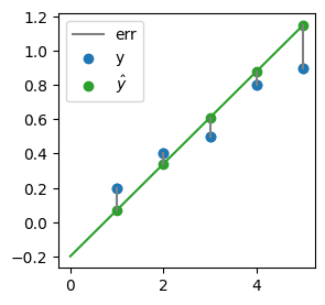
As a fitness metric, we could use the error that each model makes. For each observed datum, the error is:
where \( \hat{y}_i\) is the model prediction for the corresponding \(x_{i}\):
plt.figure(figsize=(3,3))

yhat_1 = funct(np.array(X), alphas[1], betas[1]) # model predictions (dots)
y_model_1 = funct(xx, alphas[1], betas[1]) # just for plotting the model (line)

plt.plot(xx, y_model_1, c='C2')
errs = plt.plot((X, X), (y, yhat_1), c='grey', label='err')
plt.setp(errs[1:], label="_")
plt.scatter(X, y, label='y', c='C0')
plt.scatter(X, yhat_1, label=r'$\hat{y}$', c='C2')

plt.scatter(X, y)
plt.legend()
plt.show()
\(\rightarrow\) So what about picking the \(\alpha\) and \(\beta\) that minimize the errors?
It’s easier if we use single number to minimize, so, we can consider the “sum of errors”:
Q: But minimizing this has a problem. Can you guess?
[Spoiler] (click here to expand)
\(\rightarrow\) For reasonable residuals, it averages to zero \(\rightarrow\) Difficult to minimize!
We consider the sum of squares:
and hence the Least Squares Method:
The best-fitting parameters (=model) are those that minimize the sum of squares of the errors
IMPORTANT:
The Least Squares method is only one possible optimization method.
As we will see over and over again during this course, there are other definitions of “best fitting model” (e.g. the one that minimizes the absolute error), as well as countless algorithms to find such optimum.
Yet, LS is a very good example to start with, to get the general intuition behind otpimization.
8. Fitting a line via Ordinary Least Squares (OLS)#
The linear case offers the simplest application of LS fitting, which goes under tha name of Ordinary Least Squares (OLS).
Simple \(\rightarrow\) We can solve this analytically (no approximations, no iterations, computationally fast).
8.1. Problem definition#
See this wikipedia article on OLS for the formalism/nomenclature.
We first need to generalize to \(p\) dimensions \(\rightarrow\) now, each \(X_i\) for sample \(i\) is not a single feature (as before), but an array of features:
So, if we have \(n\) samples, each having \(p\) dimensions, the data matrix is:

|
NOTE: Samples are along columns, in this notation.
However, the target variable is still one-dimensional:
|
|
Now, for the model \(-\) In the 1D cases we said it was:
Generalizing to \(p\) dimensions, one could say that the multi-dimensional model should be of the form:
… where “const” plays the role of \(\beta\) in the 1D case, and instead of using \(\alpha\), \(\beta\), \(\gamma\), etc., we just use \(\beta_1\), \(\beta_2\), \(\beta_3\), not to run out of Greek letters!
We can forget about the const with a small trick, without losing generalization (again, see the wikipedia OLS article) \(-\) so our generalized multi-dimensional linear model becomes:
But, to be formally precise, we should add the index \(i\), because this must old true for every data point \(i\):
or, in vector notation:
for each point \(i\). In matrix notation we can represent the equations for all points in one go:

|
8.2. Solution#
See this wikipedia article on Least squares for the derivation.
The solution is obtained by:
Writing the squares in a convenient form
Finding the minimizer by searching where the derivative of \(S(\pmb{\beta})\) equals 0
IMPORTANT: We want to minimize \(S(\pmb{\beta})\) with respect to \(\pmb{\beta}\), not \(\pmb{X}\) !
\(\rightarrow\) i.e., we are looking for the best parameter set \(\hat{\pmb{\beta}}\) that minimizes the squared errors:\(\pmb{\beta} = \operatorname{argmin_\beta} S(\pmb{\beta})\)
simplifying, and moving terms around it follows:
Extremely simple
But is it computationlly fast?
Inverting a matrix (in our case, (\(\pmb{X}^T\pmb{X})^{-1}\)) is a “heavy lifting” job for a computer.
\(\rightarrow\) complexity: \(\mathcal{O}(n^3)\)
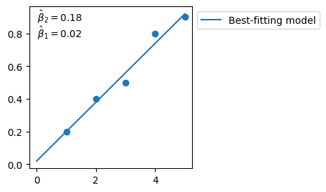
8.3. In python#
We will use numpy.linalg.lstsq to fit:
to the data seen above (notice that now we call every parameter as “\(\beta_{<number>}\)”, as for the generic multi-dimensional case).
# Same data as above:
X = np.array([1, 2, 3, 4, 5])
y = np.array([0.2, 0.4, 0.5, 0.8, 0.9])

from numpy.linalg import lstsq

X_prime = np.vstack([X, np.ones(len(X))]).T
'''
What is this line doing?! Adding a row of `1`s to our data?! Why?

Remember, above, when we said that we can "hide" the constant in:
    y = beta*X + const
using a trick?

The trick it is to create a "fake", additional feature in X, and fill it
with ones.  This will play the role of the constant.

See the links above, as well as the `np.linalg.lstsq` documentation, here:
    https://numpy.org/doc/stable/reference/generated/numpy.linalg.lstsq.html
''';

beta_2_hat, beta_1_hat = np.linalg.lstsq(X_prime, y, rcond=None)[0]
# best-fitting parameters

fig, ax = plt.subplots(figsize=(3,3), ncols=1, nrows=1)
plt.scatter(X, y)
plt.plot(xx, beta_2_hat*xx + beta_1_hat, 'C0', label='Best-fitting model')
plt.text(.05, .99, '$\\hat{\\beta}_2 = %.2f$' % beta_2_hat, ha='left', va='top', transform=ax.transAxes)
plt.text(.05, .89, '$\\hat{\\beta}_1 = %.2f$' % beta_1_hat, ha='left', va='top', transform=ax.transAxes)
plt.legend(bbox_to_anchor=(1, 1))
plt.show()
8.4. In python - an easier library#
Ok, numpy.linalg.lstsq is very educational because it solves the OLS problem algebraically, just like but in Equation 1.
But \(-\) as you have seen \(-\) it has a clumsy usage.
For practical purposes, we will now on use the much more intuitive and flexible lmfit.
NOTE: Internally, it uses by default a different algorithm to solve the least-squares problem (see later: “Levemberg-Marquardt”), but we pretend not, for now.
from lmfit import Model

def model_func(x, beta_1, beta_2):
    y = beta_2*x + beta_1
    return y

# Create an lmfit `Model` object:
model = Model(model_func)

# Invoking the `fit()` method, which returns the object `result`:
result = model.fit(y, x=X, beta_1=0, beta_2=1)
'''
Notice that here we are providing some initial guess for `beta_1` and `beta_2`,
this is only because this library is using the Levemberg-Marquardt algorithm.

In reality OLS doesn't need initial guesses when using the algebraic solution,
as demonstrated above by using `np.linalg.lstsq`, which properly solves OLS.

We will see later why Levemberg-Marquardt requires initial guesses.
'''

# Retrieving best-fit parameters:
beta_1_hat = result.params['beta_1'].value
beta_2_hat = result.params['beta_2'].value

xx = np.linspace(0 , np.max(X), 100)
'''Notice that `xx` is not the same as `X` (the data), but just
an array of equally spaced values that we use for plotting purposes.'''

fig, ax = plt.subplots(figsize=(3,3), ncols=1, nrows=1)
plt.scatter(X, y)
plt.plot(xx, beta_2_hat*xx + beta_1_hat, 'C0', label='Best-fitting model')
plt.text(.05, .99, '$\\hat{\\beta}_2 = %.2f$' % beta_2_hat, ha='left', va='top', transform=ax.transAxes)
plt.text(.05, .89, '$\\hat{\\beta}_1 = %.2f$' % beta_1_hat, ha='left', va='top', transform=ax.transAxes)
plt.legend(bbox_to_anchor=(1, 1))
plt.show()

Exercise [30 min]
Objective: Evaluate the best-fit model to some data. You will have to assume a model, and then run the Least-Squares minimization on the provided data.
The final goal is to observe what happens when you apply the model to new, “test” data.
Dataset: The following one.
# Loading and plotting data:
import tarfile
import io
from matplotlib import pyplot as plt
import numpy as np

tar = tarfile.open("data/C02_data_ex1.tar.gz", "r:gz")

def convert_and_load(file):
    with io.BytesIO(file.read()) as f:
        return np.load(f)

for member in tar.getmembers():
    file = tar.extractfile(member)
    if member.name == 'X_train.npy': X_train = convert_and_load(file)
    if member.name == 'y_train.npy': y_train = convert_and_load(file)
    if member.name == 'X_test.npy':  X_test  = convert_and_load(file)
    if member.name == 'y_test.npy':  y_test  = convert_and_load(file)

plt.figure(figsize=(10, 4))
plt.scatter(X_train, y_train, label='train', c='C0', s=15)
plt.scatter(X_test,  y_test,  label='test',  c='C1', s=15)
plt.xlabel('X')
plt.ylabel('y')
plt.title('train/test split')
plt.legend(loc='center left', bbox_to_anchor=(1, 0.5))
plt.show()
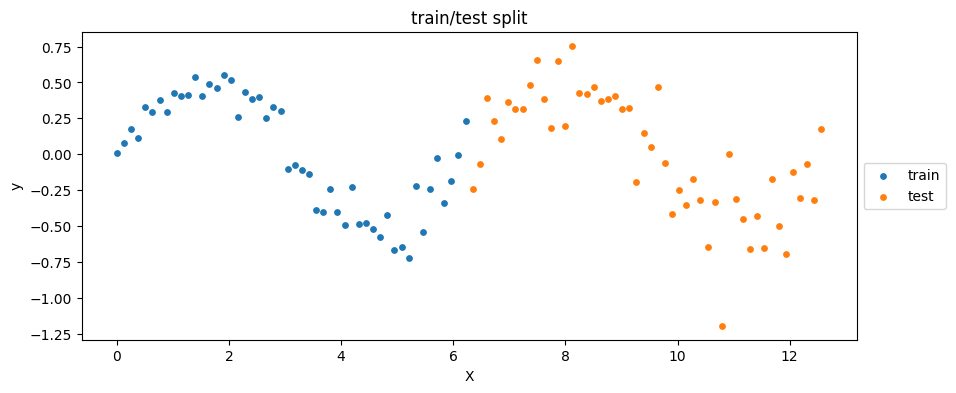
Task: In particular, you will have to:
Look at the data and assume a model
Use only the “train” data to perform the LS minimization to find the best model
Using the best model, calculate and plot the model predictions on the “train” data
Calculate and plot the model predictions on the “test” data
Calculate the squares of errors for the “train” (\(S_{train}\)) and “test” (\(S_{test}\)) data
Now compare the two squares of errors \(\rightarrow\) What do you notice?
Hints:
For task 4 \(-\) To get the squares of errors you can simply calculate: $\( S_{train} = \sum_i (y_i - \hat{y}_i)^2 ~~~~~ \forall i \in train\)$
Notice that \(-\) once the model has been fit \(-\) \(S_{train}\) is effectively the minimized Least Squares.
But what about \( S_{test} \)?
Our solution
from lmfit import Model

# 1. Assuming a sinusoidal model
def model_func(x, beta_1):
    y = beta_1*np.sin(x)
    return y

# 2. Using only the "_train_" data to perform the LS minimization

# Create an lmfit `Model` object:
model = Model(model_func)

# Invoking the `fit()` method, which returns the object `result`:
result = model.fit(y_train, x=X_train, beta_1=0)

# Retrieving best-fit parameters:
beta_1_hat = result.params['beta_1'].value

# 3. Calculating and plotting the model predictions on the "_train_" data
# 4. Calculating and plotting the model predictions on the "_test_" data
# Predictions of the model for train/test:
yhat_train = model_func(X_train, beta_1_hat)
yhat_test  = model_func(X_test,  beta_1_hat)

xx = np.linspace(0 ,np.max(X_test), 100)
'''Notice that `xx` is not the same as `X` (the data), but just
an array of equally spaced values that we use for plotting purposes.'''

plt.figure(figsize=(10, 4))
# Data:
plt.scatter(X_train, y_train, label='train', c='C0', s=15)
plt.scatter(X_test,  y_test,  label='test',  c='C1', s=15)
# Model:
plt.plot(xx, model_func(xx, beta_1_hat), label='model', c='grey', lw=2)
# Train predictions:
plt.scatter(X_train, yhat_train, label='$\hat{y}_{train}$', c='C2', s=15)
# Test predictions:
plt.scatter(X_test,  yhat_test,  label='$\hat{y}_{test}$',  c='C3', s=15)
#
plt.xlabel('X')
plt.ylabel('y')
plt.title('Best-fitting model')
plt.legend(loc='center left', bbox_to_anchor=(1, 0.5))
plt.show()
# 5. Calculating squares of errors for the "_train_" and "_test_":
S_train = np.sum( (yhat_train - y_train)**2 )
S_test  = np.sum( (yhat_test - y_test)**2 )

# 6. Now comparing the two squares:
print("S_train: %.2f | S_test: %.2f" % (S_train, S_test))
S_train: 0.68 | S_test: 2.43
\(S_{test}\) is way larger than \(S_{train}\) \(\rightarrow\) overfitting
This is to be expected because the model has been trained on \(X_{train}\), and, as you can see, \(X_{test}\) shows larger variance.
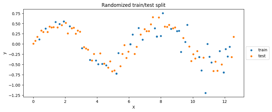
Q: What could we do to obtain a more balanced model (i.e., a model with similar performance on train and test data)?
[Spoiler] (click here to expand)
\(\rightarrow\) Shuffle the data!
'''Merging train and test data, first.'''
X = np.concatenate((X_train, X_test))
y = np.concatenate((y_train, y_test))

'''
Now performing a random split of the merged data.
Re-running this block will generate a new, randomized split.
'''
idxs_train_ = np.random.choice(np.arange((len(X))), size=len(X_train))
# ^here we pick at random some train indexes from the merged `X`
idxs_test_ = list(set(np.arange((len(X)))) - set(idxs_train_))
# ^here we pick the complementary indexes

X_train_ = X[idxs_train_]
y_train_ = y[idxs_train_]
X_test_ = X[idxs_test_]
y_test_ = y[idxs_test_]

plt.figure(figsize=(10, 4))
plt.scatter(X_train_, y_train_, label='train', c='C0', s=15)
plt.scatter(X_test_,  y_test_,  label='test',  c='C1', s=15)
plt.xlabel('X')
plt.ylabel('y')
plt.title('Randomized train/test split')
plt.legend(loc='center left', bbox_to_anchor=(1, 0.5))
plt.show()
'''Re-running the same fit as above on the new, randomized split.'''
from lmfit import Model

def model_func(x, beta_1):
    y = beta_1*np.sin(x)
    return y

model = Model(model_func)

result = model.fit(y_train, x=X_train, beta_1=0)

beta_1_hat = result.params['beta_1'].value

yhat_train_ = model_func(X_train_, beta_1_hat)
yhat_test_  = model_func(X_test_,  beta_1_hat)

xx = np.linspace(0 ,np.max(X), 100)

plt.figure(figsize=(10, 4))
plt.scatter(X_train_, y_train_, label='train', c='C0', s=15)
plt.scatter(X_test_,  y_test_,  label='test',  c='C1', s=15)
plt.plot(xx, model_func(xx, beta_1_hat), label='model', c='grey', lw=2)
#
plt.xlabel('X')
plt.ylabel('y')
plt.title('Best-fitting model')
plt.legend(loc='center left', bbox_to_anchor=(1, 0.5))
plt.show()

S_train = np.sum( (yhat_train_ - y_train_)**2 )
S_test  = np.sum( (yhat_test_ - y_test_)**2 )
print("S_train: %.2f | S_test: %.2f" % (S_train, S_test))
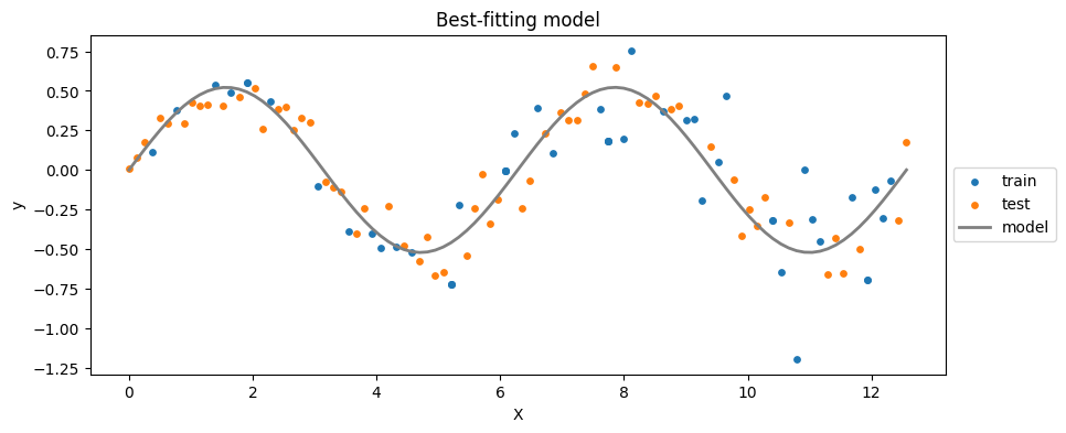
S_train: 2.84 | S_test: 0.93
9. Non-linear least squares: Levemberg-Marquardt algorithm#
We saw linear problems, i.e. when the model is linear in the parameters, e.g.:
What about the non-linear problems, i.e. when the model is not linear in the parameters, e.g.:
In general, LS not solvable algebraically \(\rightarrow\) Need to converge to the solution!
9.1. Brute-force approach (spoiler: doesn’t work!)#
Objective: The taks is \(-\) as usual \(-\) to find the parameter set \(\hat{\pmb{\beta}}\) that minimizes the sum of squares \(S(\pmb{\beta})\).
So, let’s say that we have a model of the type:
and we want to find \(\hat{\pmb{\beta}} = (\hat{\beta_1}, \hat{\beta_2})\) that minimizes \(S(\beta_1, \beta_2)\).
Let’s assume we could potentially explore all possible parameter combinations.
For each given \((\bar{\beta}_1, \bar{\beta_2})\) set, we:
Create a the corresponding model: \(\bar{y}_{pred} = \bar{\beta}_1e^{\bar{\beta}_2 x} \)
Calculate \(S(\bar{\beta}_1, \bar{\beta}_2) = \sum_i^{n}(\bar{y}_{i, pred} - y_{i, obs})^2\)
… and repeat ad infinitum.
\(\rightarrow\) Then, we could hypothetically map the whole \(S(\beta_1, \beta_2)\) space:
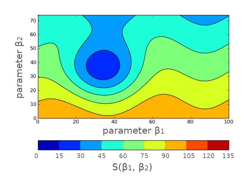
Except that this will take forever!
9.2. Iterative approach (now we are talking!)#
Instead, we may want to converge to the best solution \(\hat{\pmb{\beta}} = (\hat{\beta_1}, \hat{\beta_2})\).
(possibly in a fast way)
We will accept a compromise: approximate solution.
We start from a blank state:
|
|
Or, better, from an initial guess \((\beta^A_1, \beta^A_2)\):
(We look at the function, we had an enlightment, we used chat codes, etc.)

|
NOTE: Here we conveniently show the neighborhood around the point we pick.
Q: Where to take the next guess?
[Spoiler] (click here to expand)
What about looking at the gradient (i.e., derivative) around that point \(\rightarrow\) it points towards where the \(S(\beta_1, \beta_2)\) is decreasing.

|
Let’s follow the white rabbit and see where it leads us …
We take the next guess \((\beta^B_1, \beta^B_2)\) somewhere along the gradient:

|
Not bad! It lead us to a lower \(S(\beta_1, \beta_2)\). Let’s try again …
We take another guess somewhere along the gradient:

|
And again, and again .. until we are happy (define happy)

|
9.3. Enough with the crayons - now, math!#
NOTE: The theory in this section is taken from this wikipedia article on Levemberg-Marquardt algorithm
Let’s call: \(\hat{y}_i := f(x_i, \pmb{\beta})\) \(\leftarrow\) model value for \(x_i\)
The initial guess for the best-fit parameters is \(\pmb{\bar{\beta}}\).
The next guess is: \(\pmb{\bar{\beta}} \rightarrow \pmb{\bar{\beta}} + \pmb{\delta}\), where \(\pmb{\delta}\) is the small amount we move.
Objective: Update \(\pmb{\bar{\beta}}\) until we minimized \(S(\pmb{\beta})\)
We can use the Taylor expansion to approximate \(f(x_i, \pmb{\bar{\beta}})\) around \(\pmb{\bar{\beta}}\):
IMPORTANT: Notice that the derivative is on the parameters (\(\pmb{\beta}\)), not the data (\(x_i\))! \(\rightarrow\) We want to explore the neighborhood of \(\pmb{\bar{\beta}}\)!
We can define \(\pmb{J_i} := {\partial f(x_i, \pmb{\beta}) \over \partial\pmb{\beta}} \), so:
Algorithm:
We now need to define how much to move, to find the next gues \(\rightarrow\) \(\pmb{\delta} = ?\)
We will find it by solving the usual problem \(\rightarrow\) minimize the sum of squares.
If the next guess \(\pmb{\bar{\beta}} + \pmb{\delta}\) corresponds to a true minimum, then \(S(\pmb{\bar{\beta}} + \pmb{\delta})\) must have derivative = 0 (w/r to vector \(\pmb{\delta}\)):
Meaning: moving away from \(\pmb{\bar{\beta}} + \pmb{\delta}\) causes a worse result.
Let’s solve it, starting from the approximation of Equation 2:
$
$
Which \(-\) in vector notation \(-\) becomes:
$
$
Now we take the derivative w/r to vector \(\pmb{\delta}\) (this tables will help to follow the calculations):
$
$
.. and finally:
\(\rightarrow\) set of \(p\) linear equations (\(p\) = number of parameters) that can be solved for \(\pmb{\delta}\) !
To get to a better minimum, we can just repeat the procedure by replacing the starting point: \(\pmb{\bar{\beta}^{\prime}} = \pmb{\bar{\beta}} + \pmb{\delta}\), move to \(\pmb{\bar{\beta}^{\prime}} + \pmb{\delta}^{\prime}\), etc.
… until we are happy.
9.4. Actual Levemberg & Marquardt algorithms#
Equation 3 is known as Gauss-Newton method (1700-1800 ca.)
The Levemberg modification (1944) is:
\(\lambda\) \(\rightarrow\) damping factor
Helps for faster convergence and larger accuracy in finding the minimum
Adjusted at each iteration:
if \(S(\pmb{\beta})\) decreases rapidly \(\rightarrow\) \(\lambda\) is decreased (deceleration)
if \(S(\pmb{\beta})\) doesn’t decrease enough \(\rightarrow\) \(\lambda\) is increased (push)
9.5. Further reads#
Marquardt contribution \(\rightarrow\) wikipedia article on Levemberg-Marquardt algorithm
Stopping criteria \(\rightarrow\) wikipedia article on Levemberg-Marquardt algorithm
Shortcomings of L-M \(\rightarrow\) this blog
10. Chi-square (χ2) fitting#
Basically, it’s least squares for when data have errors on y
X = [1, 2, 3, 4, 5]
y = [0.2, 0.4, 0.5, 0.8, 0.9]
y_err= [0.1, 0.05, 0.2, 0.03, 0.2]

from matplotlib import pyplot as plt
plt.figure(figsize=(3,3))
plt.errorbar(X, y, yerr=y_err, marker="o", ls="none")
plt.show()
Instead of minimizing the sum of squares \(S(\pmb{\beta})\), we minimize the weighted average of the sum of squares \(\chi^2\):
… where the weigths are the measurement uncertainties \(\sigma_i\).
10.1. Further reads#
Why do we use the “reduced” \(\chi^2\) to compare model results (i.e., \(\chi_{\nu}^2\))? \(\rightarrow\) Andrae et al. 2010